The first time you look at a live options chain, it reads like a foreign language. Numbers everywhere — strike prices, premiums, expiration dates — and somewhere buried in there, a column labeled “IV” that nobody bothered to explain. That was the moment I realized that reading about options and actually understanding them were two completely different things.
If you’re looking to learn options trading Greeks and implied volatility through Python, the fastest path isn’t memorizing formulas — it’s building them yourself and watching them break on real data. Delta, Gamma, Theta, and Vega stop being abstract symbols the second you implement Black-Scholes from scratch and see how each partial derivative behaves as price, time, or volatility shifts. That’s the knowledge that actually sticks.
- Greek sensitivity only makes sense when you see it move — implement it in code before reading another definition
- Implied volatility is not historical volatility; confusing them is the most expensive mistake beginners make
- An iron condor looks safe on paper until you model it against real IV data from an exchange
What Options Greeks Actually Measure
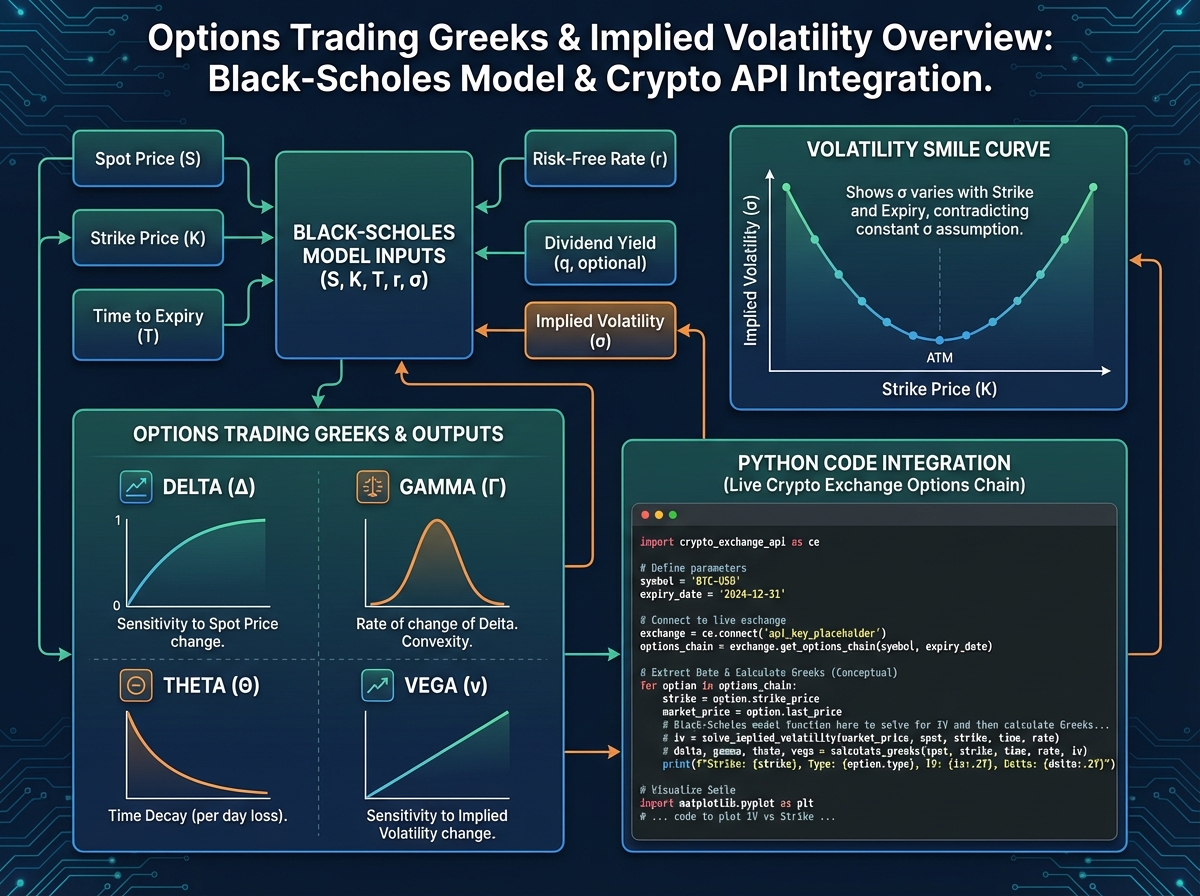
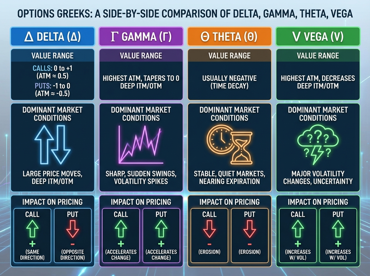
Greeks are sensitivity measures — each one tells you how an option’s price responds to a specific change in market conditions. Delta measures how much the option moves when the underlying moves by one unit. Gamma measures how fast Delta itself changes. Theta captures daily time decay, and Vega shows how sensitive the option is to changes in implied volatility.
For traders moving from theory to live markets, the key distinction is between intrinsic value (what an option is worth if exercised right now) and extrinsic value (the time and volatility premium baked into the price). An at-the-money option is almost entirely extrinsic value — which means Theta and Vega dominate its behavior, not Delta.
| Greek | Measures | Key Behavior |
|---|---|---|
| Delta | Price sensitivity to underlying move | Ranges 0–1 for calls, 0 to -1 for puts |
| Gamma | Rate of change of Delta | Highest near ATM, spikes near expiry |
| Theta | Time decay per day | Always negative for long options |
| Vega | Sensitivity to 1% change in IV | Highest for long-dated ATM options |
Three things that surprise almost every beginner:
- Theta decay is not linear — it accelerates sharply in the final two weeks before expiration
- A high Vega position can lose money even when you’re directionally correct
- Gamma risk near expiry can wipe a position that looked perfectly hedged the day before
How Long It Actually Takes to Go from Zero to Live Analysis
| Stage | Content | Time |
|---|---|---|
| Foundations | Options basics, terminology, moneyness, calls vs puts | 3–5 hours |
| Pricing mechanics | Intrinsic/extrinsic value, Black-Scholes intuition, Monte Carlo | 6–8 hours |
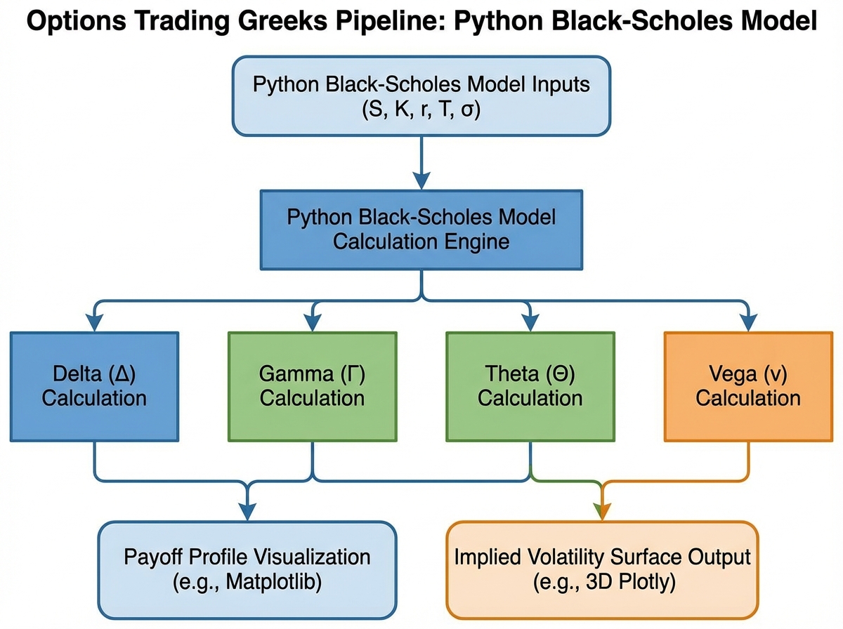
| Greeks in Python | Implementing Delta, Gamma, Theta, Vega from scratch using BS model | 5–7 hours |
| Implied volatility | Newton-Raphson, Brent’s method, volatility smile, real market IV | 4–6 hours |
| Strategy building | Covered calls, spreads, iron condors, butterflies — coded and visualized | 6–9 hours |
| Execution & risk | Slippage, order types, position sizing, risk mindset | 2–3 hours |
| Real market project | Live data from Binance/Bybit, option chain analysis | 3–5 hours |
| Total | 29–43 hours |
Order matters far more than speed here — Greeks become meaningful only after you’ve built the pricing model, and implied volatility only clicks after you’ve already used Black-Scholes to calculate theoretical prices. If you’re moving slower than the estimate above, that’s usually a sign you’re going deeper on the right things.

The Part Where Most People Get Lost First
Everyone starts with the terminology — calls, puts, strike price, expiration — and it all feels manageable. Then they hit “moneyness” and suddenly need to hold three states in their head simultaneously: in-the-money, at-the-money, out-of-the-money, and how each affects intrinsic and extrinsic value differently. The instinct is to move on before that distinction is solid. That’s the first mistake, and it costs you later.
The concept that actually unlocks options is understanding that you’re not buying a stock — you’re buying optionality. The premium you pay is compensation to the seller for the uncertainty they’re absorbing. Once that framing lands, things like why OTM options are cheaper, why volatility inflates premiums, and why time decay only hurts the buyer start making intuitive sense rather than mechanical sense.
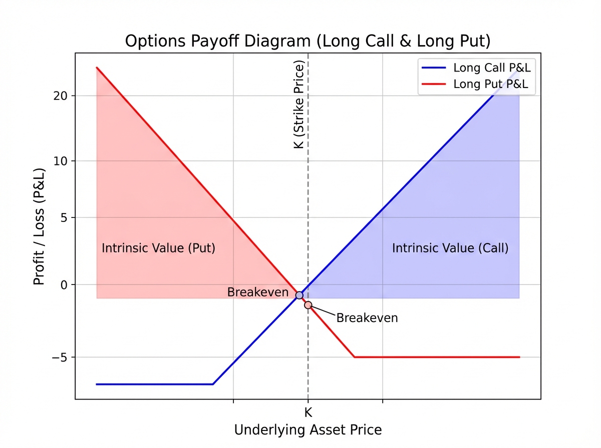
Visualizing payoff profiles in Python at this stage is what makes the difference. Plotting a call’s P&L curve across a range of underlying prices — and watching it go from flat to sharply positive past the strike — turns an abstract concept into something you can manipulate and test. By the time you move to Greeks, you already have an intuition for what you’re measuring.
Where Black-Scholes Actually Becomes Useful
The Black-Scholes model gets treated like a magic formula in most textbooks — plug in five inputs, get a price. That framing is useless for actually trading. What matters is understanding which inputs drive the price most in different scenarios, and that only becomes clear when you implement it yourself.
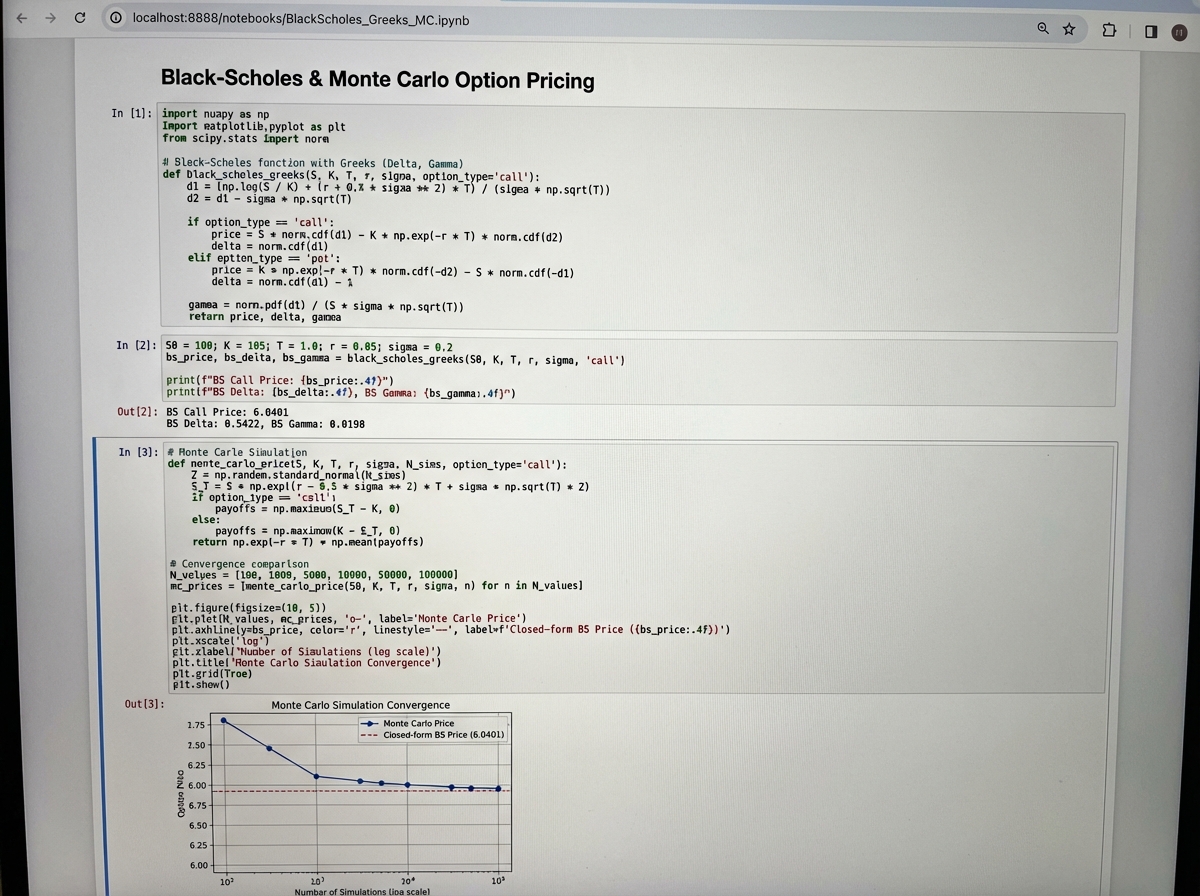
Building the model in Python means working through why the formula uses a log-normal distribution for price returns, why time appears as a square root, and what the d1 and d2 terms are actually computing. When you then derive Delta as the partial derivative with respect to the underlying price, it stops being a number you look up and becomes something you calculated — and that changes how you trust it.
The real turning point is running a Monte Carlo simulation for option pricing alongside the closed-form Black-Scholes result and watching them converge. That moment — seeing two completely different methods arrive at nearly the same number — is when the model stops feeling like a black box and starts feeling like a framework you can interrogate.
What Implied Volatility Really Is (and Why It Trips Everyone Up)
The single biggest mistake people make when learning options trading Greeks is treating implied volatility like a property of the underlying asset. It isn’t. IV is the volatility that, when plugged into Black-Scholes, makes the model’s theoretical price match the actual market price. It lives in the option, not the stock.
This distinction changes everything about strategy selection. When IV is elevated — before earnings, before a major macro event — options are expensive not because the underlying is moving more, but because the market is pricing in the expectation that it might. Selling premium in high-IV environments and buying in low-IV environments is the core logic behind an entire class of strategies. None of that is obvious until you’ve built an IV solver yourself.
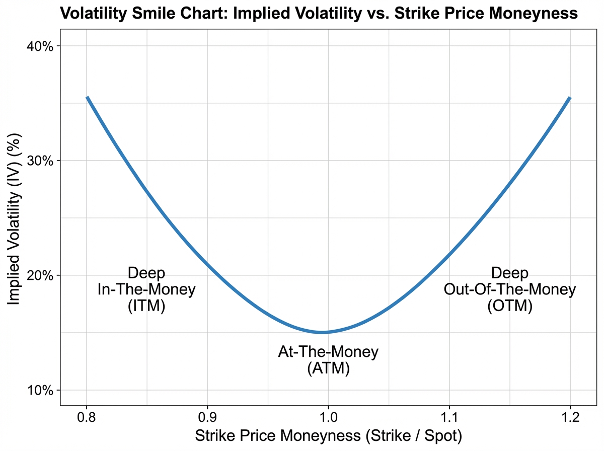
Implementing Newton-Raphson to solve for IV numerically is where Python-driven options learning becomes genuinely powerful. You start with a market price from a real exchange, invert the Black-Scholes formula iteratively, and recover the implied volatility the market is embedding in that price. When you then plot IV across strikes and see the volatility smile — the characteristic curve that shows IV is higher for deep OTM options — you understand immediately why Black-Scholes is a starting point, not an endpoint.
Building Real Strategies and Watching Greeks Interact
Covered calls and protective puts are the entry points for strategy logic — they’re simple enough to reason about in your head, but complex enough to reveal how Greeks interact once you model them. A covered call caps your upside while collecting premium; a protective put costs premium but floors your downside. Modeling them side-by-side in Python and plotting both payoff curves on the same chart makes the trade-off viscerally clear.
Vertical spreads are where strategy thinking gets interesting. A bull call spread — buying a lower strike call and selling a higher one — limits both your maximum gain and maximum loss. The sold call offsets some of the premium you paid, but it also caps your Vega exposure. When you implement this in Python and observe how Theta affects the two legs differently at different points in time, you realize that multi-leg strategies aren’t just about payoff shapes: they’re about managing how Greeks evolve as the trade ages.
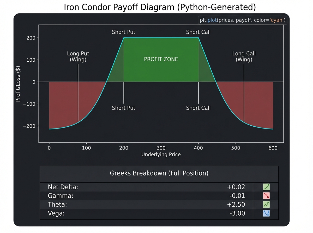
Iron condors and butterflies are where everything comes together. An iron condor sells a strangle and buys wings for protection — it’s a bet that the underlying stays range-bound. Modeling one against real IV data from a crypto exchange reveals something that paper trading never would: the theoretical maximum profit looks clean on the payoff diagram, but the live bid-ask spreads and actual IV levels mean the real entry cost is often higher and the actual edge narrower than the diagram suggests.
Execution Is Where Theory Gets Humbled
The gap between a beautiful payoff diagram and a real trade is filled with slippage, bid-ask spreads, and liquidity constraints. Placing a market order on an illiquid options contract can immediately push you 2–3% against your theoretical entry price — a problem that never appears when you’re modeling in Python against clean historical data.
Limit orders solve most of this, but they introduce a different problem: partial fills. A multi-leg strategy where only two of four legs fill creates a naked exposure you didn’t intend. Understanding order types in the context of options execution — and knowing which leg to fill first — is the kind of operational knowledge that experienced traders have accumulated through expensive mistakes.
Position sizing under a risk mindset means thinking about how much capital you can afford to have in a single Greek exposure, not just how much you’re willing to lose on a trade. A portfolio of small iron condors can aggregate into a dangerously short-Vega position without you realizing it — especially when all your positions share the same underlying or the same expiry cycle.

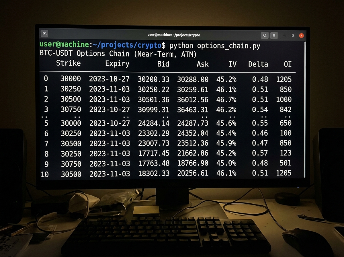
Reading a Live Option Chain Without Getting Overwhelmed
Pulling a live options chain from Binance or Bybit and making sense of it is the moment where all the prior work either pays off or exposes gaps. The raw chain is dense — dozens of strikes, multiple expiries, bid-ask spreads, open interest, and IV columns all competing for attention. Structuring it systematically in Python, filtering by expiry and moneyness, and computing Greeks across the chain turns a wall of numbers into a readable picture.
The most useful single view is a cross-section of IV by strike — which immediately shows you whether the volatility smile is symmetric (typical in equity index options) or skewed (common in crypto, where the demand for downside protection is asymmetric). From there, identifying which strikes are liquid enough to actually trade, and which strategies fit the current IV regime, becomes a structured decision rather than a guess.
This is also where reverse-engineering option prices becomes a practical skill. Given a quoted market price on Bitcoin options, recovering the implied volatility and comparing it to your model’s theoretical IV tells you whether the market is pricing in more or less uncertainty than your model expects — and that differential is where actionable analysis lives.
What You Can Actually Do With This Now
Looking back, the knowledge that compounds fastest isn’t the formulas — it’s the habit of building things in code and testing them against real prices. Every abstraction in options trading has a concrete implementation behind it, and finding that implementation is what converts theory into genuine fluency.
Here’s what to act on immediately:
- Implement Black-Scholes in Python from scratch without copying code — typing every line forces you to understand what each variable represents in a way that running someone else’s notebook never will.
- Calculate all four major Greeks for a single option position and watch them change as you vary one input at a time — this builds the intuition for how Delta, Gamma, Theta, and Vega interact before you need to manage them live.
- Build an IV solver using Newton-Raphson and test it against a real market price from a crypto exchange — this grounds implied volatility in something observable rather than theoretical.
- Plot the volatility smile for a real options chain — seeing IV curve by strike shows you instantly whether the market is pricing tail risk asymmetrically.
- Model one multi-leg strategy — start with a bull call spread — and compute the net Greeks for the full position — this reveals how selling one leg changes not just your payoff but your entire risk profile.
- Pull a live options chain and filter it down to the three most liquid at-the-money strikes — practice reading the chain before you ever consider placing a trade.
- Run a Monte Carlo simulation on a single option and compare it to your Black-Scholes price — the convergence (or divergence) tells you something real about model assumptions.
- Stress-test one strategy by simulating what happens to P&L if IV spikes 20% overnight — Vega exposure only becomes tangible when you see it in dollar terms against a position you’ve modeled yourself.
Leave a Reply