The first time you try to backtest a trading idea, you probably do what most people do — paste price data into a spreadsheet, eyeball some moving averages, and convince yourself the strategy works. Then you try it live, and it doesn’t. That gap between “it looked good on paper” and “it failed in real conditions” is exactly what serious backtesting is designed to close.
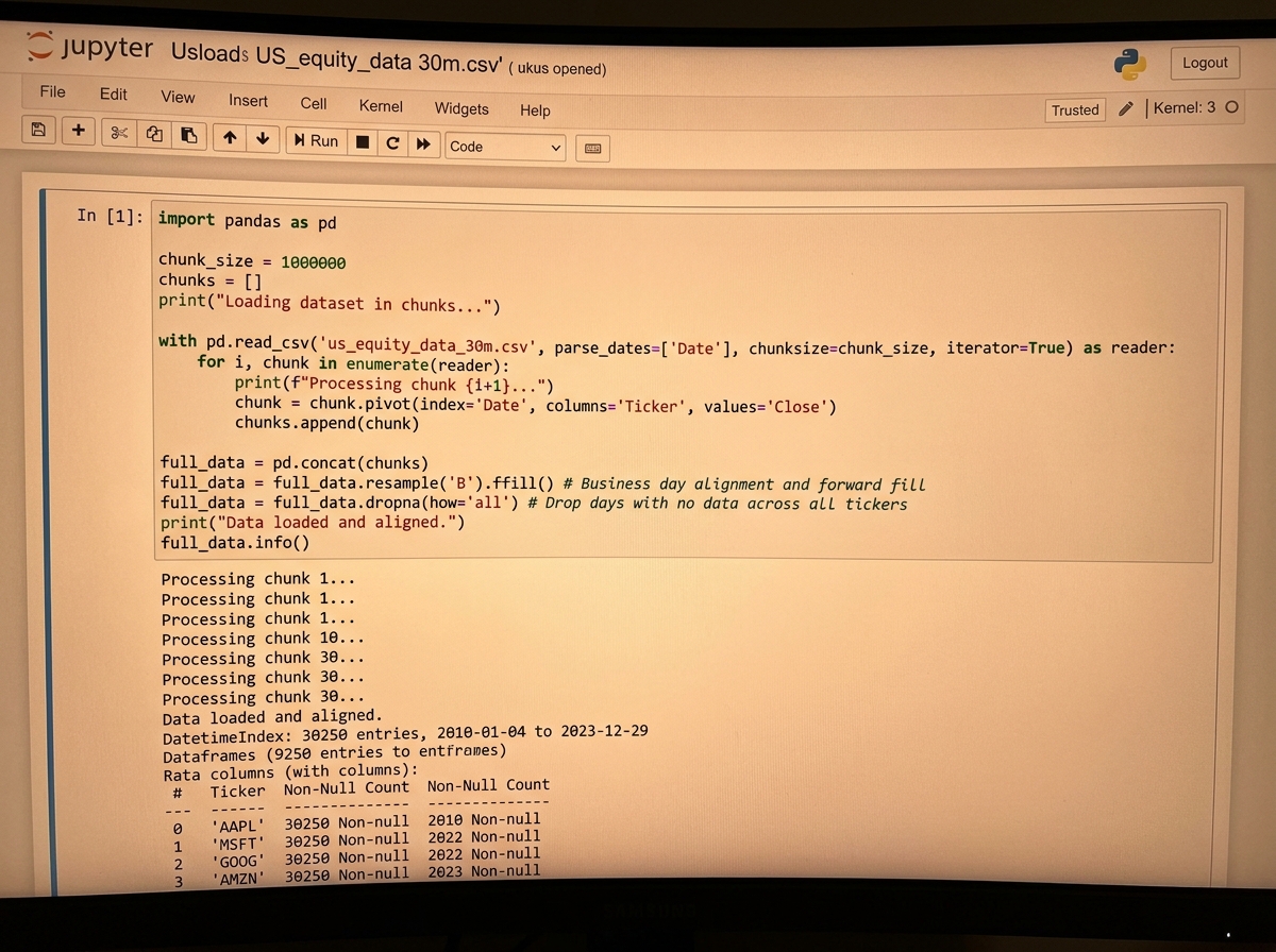
If you’re looking to learn quantitative trading backtesting in Python, the honest answer is this: you need to build your own backtester before you trust any third-party engine. Off-the-shelf tools hide assumptions about slippage, position sizing, and execution logic that quietly distort your results. Building from scratch forces you to confront every one of those assumptions head-on. With Python and a proper dataset — we’re talking over 30 million rows of US equity data spanning two decades — you can run strategies against real market conditions, not simulated toy examples.
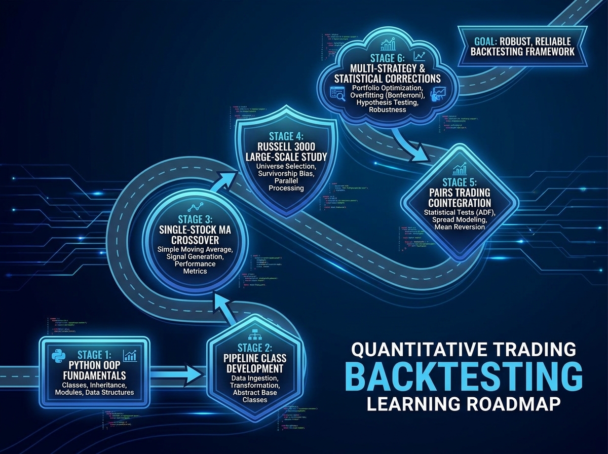
- Backtesting from scratch is more valuable than using pre-built libraries because you understand exactly what your engine assumes and where it can fail.
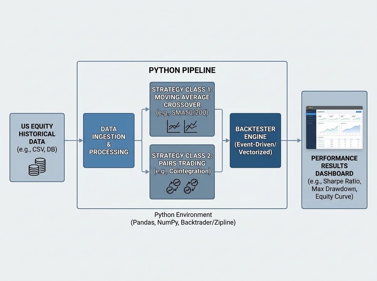
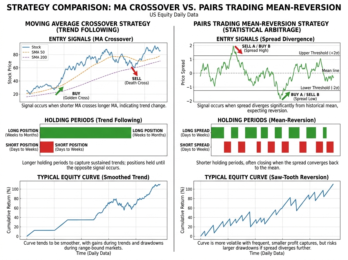
- Moving average crossover and pairs trading are the two workhorses of systematic equity trading — learning to backtest both gives you a complete foundation for almost any mean-reversion or trend-following idea.
- Large-scale simulation across hundreds of stocks, not just one ticker, is what separates a backtest that holds up from one that just got lucky on TSLA.
What Backtesting Quantitative Strategies Actually Means
Backtesting is the process of applying a trading rule to historical price data and measuring what would have happened — entry, exit, P&L, drawdown, and all. It’s not a prediction. It’s a stress test. You’re asking: “Would this idea have survived the dot-com crash, the 2008 financial crisis, and the 2020 pandemic selloff?” If the answer is no, you find out in simulation rather than with real money.
For anyone coming from a pure finance background, the Python side can feel like a wall. For anyone from a software background, the statistics — especially cointegration and time series stationarity — can feel equally foreign. The entry point that works is building the infrastructure first and layering the math on top as you need it.
| Concept | What It Is | Why It Matters in Backtesting |
|---|---|---|
| Moving Average Crossover | Signal when a short-term MA crosses a long-term MA | Trend-following entry/exit logic; easy to implement, hard to tune |
| Pairs Trading | Trade the spread between two cointegrated stocks | Mean-reversion strategy; requires statistical relationship testing |
| Cointegration (Engle-Granger) | Tests whether two non-stationary series move together long-term | The mathematical foundation for deciding which pairs to trade |
| Pipeline Class | A stock universe selector built in Python | Scales a single strategy across hundreds of tickers efficiently |
| Large-Scale Simulation | Running a strategy across all Russell 3000 stocks | Distinguishes genuine alpha from data-mining luck |
Three Things That Will Surprise You
- A strategy that works beautifully on one stock often fails on 90% of the universe.
- Cointegration between two stocks can appear and disappear within months.
- The biggest source of backtest errors is survivorship bias in your dataset, not your code.
How Long Does This Actually Take to Learn
| Stage | What You’re Building | Estimated Time |
|---|---|---|
| Setup & Data | Loading 30M-row dataset, cleaning, Pandas pipeline | 3–5 days |
| Pipeline Class | Stock universe selector with OOP structure | 2–3 days |
| Moving Average Crossover Backtester | Full class with handle_data, backtest, get_results methods | 5–7 days |
| Long-Term Study (Russell 3000 vs SPY) | Running strategy across an index, comparing high/low volatility stocks | 3–4 days |
| Pairs Trading Setup & Orders Class | Spread calculation, order logic, cointegration testing | 5–7 days |
| Pairs Trading Backtester | Full multi-class backtester with large-scale simulation | 7–10 days |
| Multi-Testing & Corrections | Multiple hypothesis testing, strategy comparison | 3–5 days |
| Total | Full working backtest framework with two strategies | 4–6 weeks |
The order in which you build these pieces matters far more than how fast you move. You cannot debug a pairs trading backtester you don’t understand at the class level, and you can’t understand the class level if you skipped the pipeline. Being slower than this estimate is completely normal — the sessions where you spend three hours tracing a bug in your handle_data method are the ones where the actual learning happens.
Getting the Data Right Before You Write a Single Strategy
Most people skip straight to coding the strategy. That’s the single biggest mistake in quantitative trading, and almost everyone makes it. Bad data produces confident-looking results that are entirely fictional. Survivorship bias alone — the fact that your dataset might only include stocks that still exist today — can make a losing strategy look like a winner by excluding all the companies that went bankrupt.
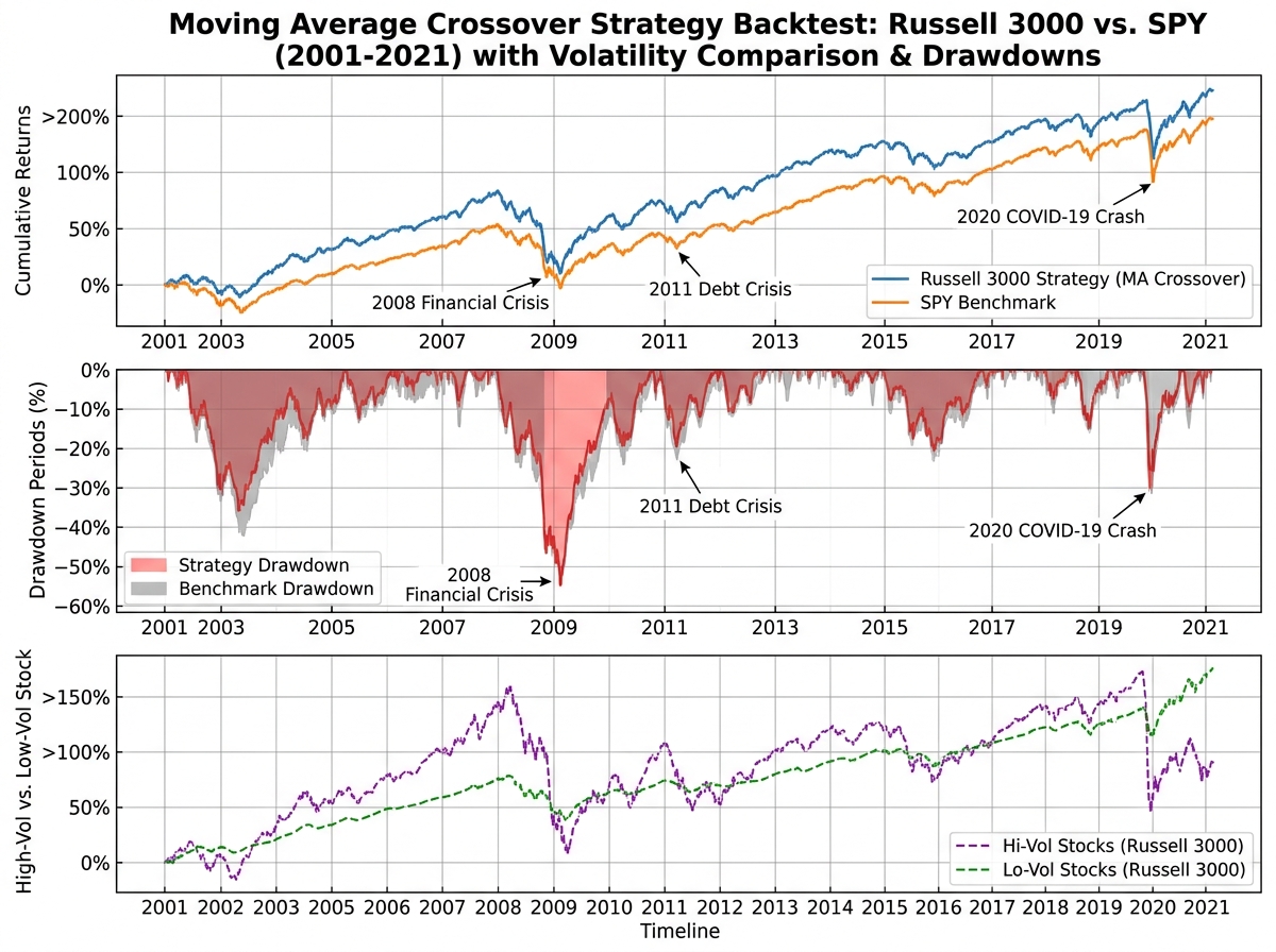
Working with a dataset that spans 2001 to 2021 and covers all tradable US equities means you’re running your strategy through periods that break most amateur systems: the 2001-2002 dot-com unwind, the 2008 credit crisis, the 2020 crash and recovery. A strategy that shows a positive Sharpe ratio across all of that deserves attention. One that was only tested on the last bull run does not.
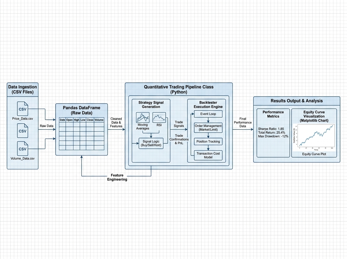
The practical work here is unglamorous. You learn to load massive files efficiently using chunked reads in Pandas, handle missing prices from trading halts, align dates across multiple tickers, and build a pipeline class that filters your universe before any strategy logic runs. None of this feels like trading. All of it determines whether your results mean anything.
Building the Moving Average Crossover Backtester
The crossover strategy is the right place to start — not because it’s profitable, but because it’s simple enough that when something breaks, you can reason about exactly why. You’re generating a signal when a short-window moving average crosses above a long-window moving average and exiting when it crosses back. The logic fits in your head, which means your bugs are structural, not conceptual.
The architecture that makes this work in Python is a class-based design with three distinct methods: handle_data, which processes each new bar of price data; backtest, which runs the strategy forward through time; and get_results, which calculates your performance metrics after the run. Separating these three responsibilities is the OOP lesson that every quantitative developer learns eventually — usually after building one giant function that’s impossible to debug.
Once the single-stock version works on something like TSLA, the real test is scaling it to the entire Russell 3000. Running it across thousands of stocks over 20 years with Joblib for parallel execution is where you stop thinking like a hobby coder and start thinking like a quant. The results at this scale are humbling in the right way: the strategy performs very differently on high-volatility versus low-volatility stocks, and that difference tells you something important about what the signal is actually capturing.
For more context on Python’s core mechanics before diving into class-based architecture, Python and Excel Integration covers Pandas fundamentals that transfer directly to backtesting work.
When Pairs Trading Finally Makes Sense
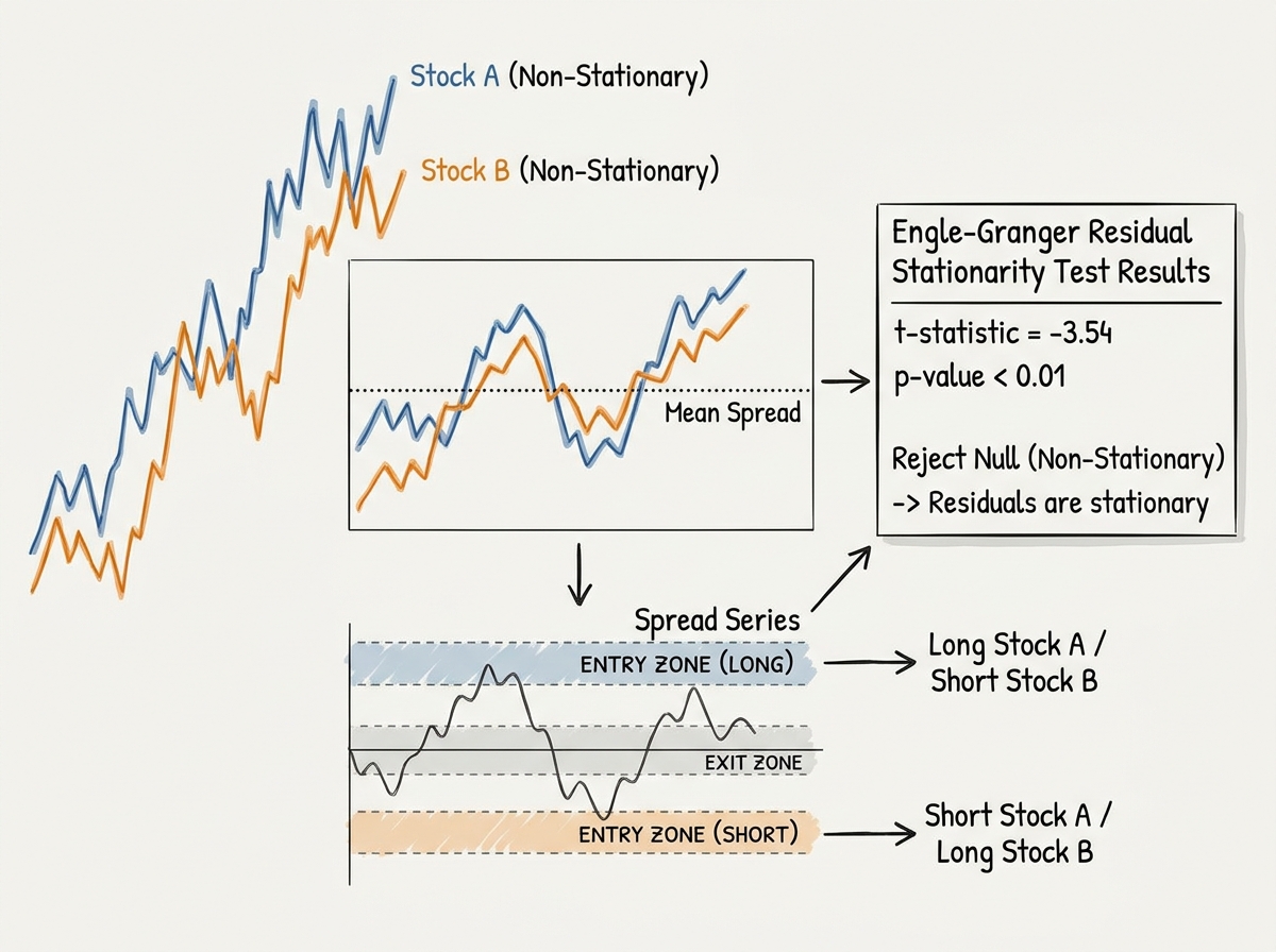
Pairs trading sounds intuitive: find two stocks that move together, and when they diverge, bet that they’ll converge again. What you don’t understand at first is that “move together” is doing enormous mathematical work in that sentence. Two stocks can be correlated — moving in the same direction on most days — without being cointegrated, and only cointegration gives you the statistical guarantee of mean reversion that makes the trade valid.
The Engle-Granger approach to testing cointegration is where the math gets real. You’re running a regression between two price series, saving the residuals, and then testing whether those residuals are stationary using an augmented Dickey-Fuller test. If they are, the spread between the two stocks is mean-reverting, and you have a mathematical foundation for a pairs trade. If they aren’t, you have two stocks that looked related but aren’t — and trading them as a pair will eventually cost you.
The Orders class is where the strategy becomes executable. You define your entry threshold (how wide does the spread need to get before you trade?), your exit threshold (how close to the mean before you close?), and your position sizing. Getting this logic clean — separating the signal generation from the order management from the position tracking — is what the multi-class structure of the pairs trading backtester is teaching you underneath the trading strategy itself.
Large-Scale Simulation and Why One Backtest Proves Nothing
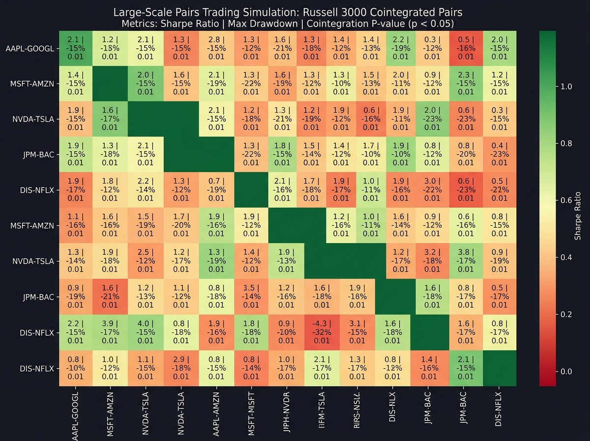
Running a pairs trading strategy on one hand-picked pair and showing that it made money is not a backtest. It’s a success story with hindsight. The moment you scale to a large-scale simulation — running cointegration tests on every possible pair in your universe, then backtesting every cointegrated pair — is the moment you see what your strategy actually does in expectation, not in your best case.
With the pipeline class driving stock universe selection, you can systematically identify candidate pairs, run the Engle-Granger test to filter for cointegration, backtest each valid pair, and aggregate the results. What you typically find is that a small percentage of pairs generate most of the returns, many pairs that looked cointegrated in the training window break down in the test window, and the overall performance is far more modest than your hand-picked example suggested. This isn’t discouraging — it’s clarifying.
Joblib makes this computationally tractable by running backtests in parallel across your core count. Without it, simulating thousands of pairs across 20 years of daily data would take hours. With it, you get results in minutes, which means you can actually iterate on your strategy logic rather than waiting for one long run to complete.
The Multiple Testing Problem Nobody Tells You About
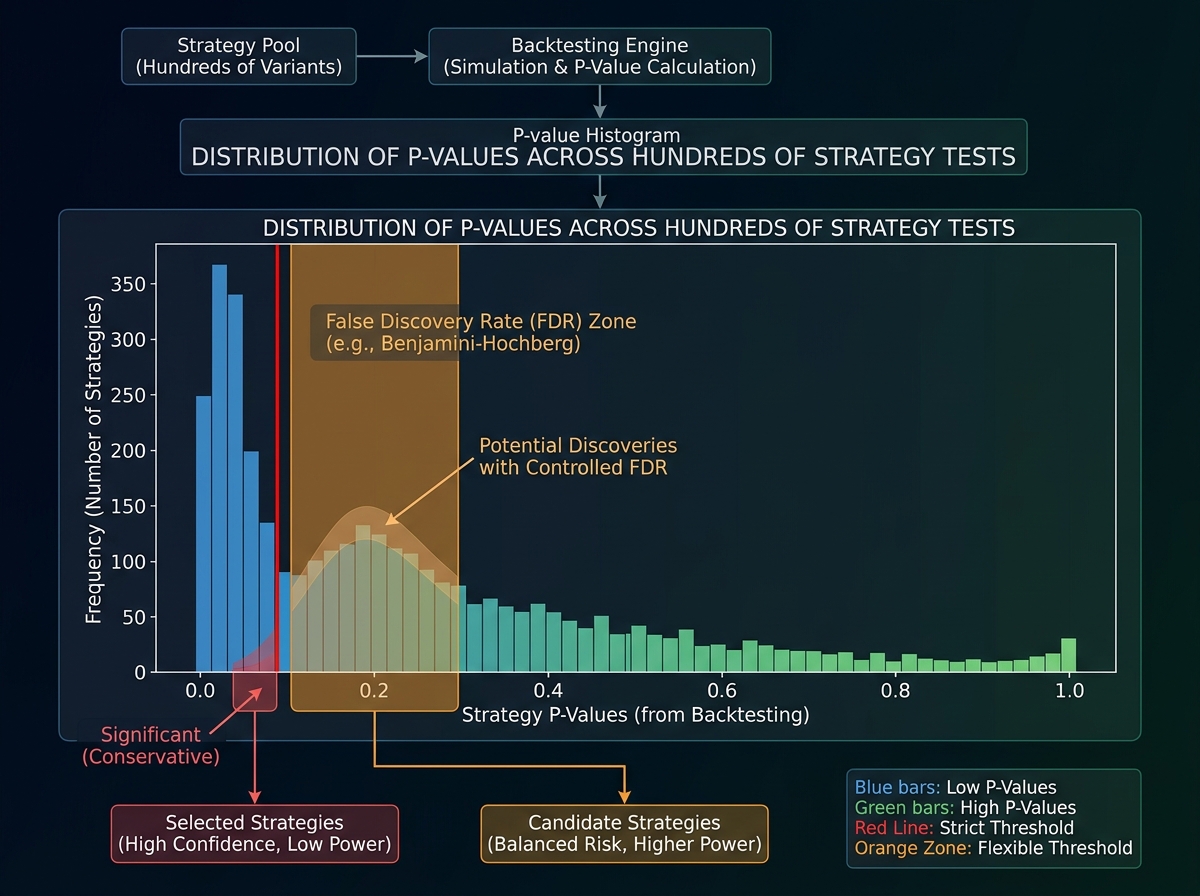
After running a large-scale simulation, you’ll have a set of strategies that showed positive returns in your test period. Here’s what most people do next: they pick the best-performing ones and declare those their final strategies. This is a serious statistical error, and it will make you lose money.
When you test hundreds of strategies, some will show positive results purely by chance. The more strategies you test, the more false positives you accumulate. This is the multiple testing problem, and there are formal corrections — Bonferroni, Benjamini-Hochberg — specifically designed to adjust your significance thresholds when you’re running many simultaneous tests. Understanding this is what separates someone doing research from someone doing data mining.
The practical implementation is a correction to your p-value thresholds that accounts for the number of tests you ran. A pairs trade that looked significant at p=0.05 when you ran one test is no longer significant at that threshold when you ran five hundred tests. Applying these corrections deflates your results back to reality — and reality, it turns out, is a much more honest place to build a trading system from.
For traders interested in how statistical signal analysis applies in live market conditions, Options Trading Greeks and Implied Volatility covers a Python-first approach to reading market structure that complements backtesting methodology.
What Changes When You Work with Real Assignment-Style Data
The final test of any quantitative framework is whether it holds up when the data is messy and someone else set the problem. Real trading firm assignments don’t give you clean daily OHLCV data and a clear objective. They give you high-frequency tick data, ask you to clean it yourself, identify the right relationship to test, and explain what trade you would put on and why.
Working through that kind of problem — sorting and cleaning tick data, determining whether a cointegrated relationship exists, designing the actual trade structure — is where every skill you built compounds. Your Pandas work handles the cleaning. Your cointegration testing framework handles the relationship identification. Your order class logic handles the trade design. The pieces connect in a way that doesn’t happen when you’re working through textbook examples with clean inputs.
This is also where the OOP investment pays off. When your backtester is a set of clean, composable classes with clear responsibilities, adapting it to a new asset class or a different data frequency is a matter of inheriting from your base class and overriding the relevant methods — not rewriting everything from scratch.
Looking back, the clearest signal that something shifted wasn’t when the backtester produced a positive Sharpe ratio — it was when I could read someone else’s strategy code and immediately understand what their handle_data method was doing and why their position sizing was probably wrong. That’s the difference between someone who ran some backtests and someone who understands backtesting.
Here’s what you can apply immediately:
- Build your crossover backtester on one stock first, then scale. Debugging a multi-ticker bug is ten times harder than debugging a single-ticker bug because you can’t eyeball the results.
- Always run your strategy on a hold-out period your eyes never touched during development. If you peeked at 2019-2021 while building your logic, those years cannot be your test set.
- Run the Engle-Granger cointegration test before assuming any pair is tradable. Correlation is not cointegration, and that distinction is worth more than anything else in pairs trading.
- Apply Bonferroni or Benjamini-Hochberg corrections any time you test more than one strategy. The number of false positives in an uncorrected multi-strategy backtest is embarrassingly large.
- Use Joblib from the start, not as an afterthought. Building the parallelization in at the pipeline level means your code scales to a full index without structural changes.
- Separate your signal generation, order logic, and results calculation into distinct classes. The pain of refactoring a monolithic function mid-project is enough to make you do it right the first time.
- Check your dataset for survivorship bias before trusting any positive result. A dataset that only includes currently listed stocks will make almost any strategy look better than it is.
- For learning Python backtesting fundamentals, How to Learn Python from Scratch gives you the Python foundation that makes OOP-based backtester architecture much easier to absorb.
Leave a Reply